Model Based Reinforcement Learning: Tutorial & Examples

Reinforcement learning (RL) is an elegant approach to building intelligent systems in which agents learn through trial and error. 

In regular operation, the agent receives its environment's state as input and, based on a policy, outputs an action. The state represents the agent's current situation, and actions are the decisions available to it. This action is applied in the environment, updating the state, which becomes the agent's input for the next step. 

With reinforcement learning, the environment also uses a reward function that encourages or penalizes depending on how optimal an action is. The function returns immediate numerical feedback evaluating each state-action pair. The state, action, and reward data are collected and used to iteratively optimize the agent policy. The best policy is one that maximizes the cumulative reward.

The key feature of model-based RL is the learning of a predictive model that allows the agent to understand how its environment behaves. This allows it to make predictions and assess actions before taking them.

The model-based reinforcement learning loop follows a consistent pattern: 

1. Collect data by taking actions
2. Train a dynamics model based on that data
3. Use the model to plan and generate actions, execute the best action, and repeat.

This article covers model-based RL from first principles, including dynamics models, planning algorithms, key challenges like compounding error and example applications in LLM training and agent development.

{{banner-large-dark-2-rle="/banners"}}

Summary of key model-based reinforcement learning concepts

Model-free vs. model-based reinforcement learning

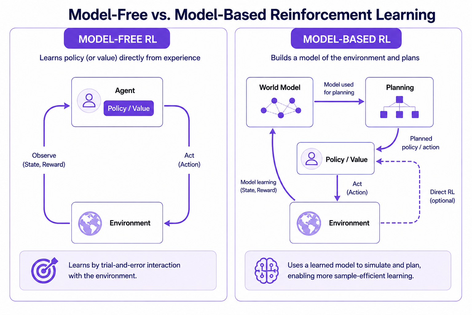
Reinforcement learning approaches are generally divided into two categories. 

1. In model-free methods, agents learn to output actions purely through trial and error. 
2. In model-based methods, agents first learn a predictive model of the environment’s dynamics and use it to inform optimal action choices.

Model-free methods 

In model-free methods like DQN, PPO, or GRPO, the policy an agent uses to generate actions is based only on learning to maximize reward, without learning an environment model. 

The primary advantage of model-free is that the solution can be deployed more flexibly even in novel environments, since there is no dynamics model to learn or maintain. However, they also require extensive interaction with the environment and can be less effective, especially if the agent’s environment and tasks are complex. 

In technical terms, model-free learning requires significantly more rollouts to achieve convergence, making the choice between the approaches a trade-off in terms of sample efficiency.

Model-based methods

Sample efficiency matters because each interaction can carry substantial cost, whether that's computational resources for LLM inference, time in a physical system, or human evaluation effort.

Model-based reinforcement learning addresses the challenges by capturing underlying dynamics and reusing them via model rollouts. Agents can extract far more efficiency from limited data. And while model-based agents are strongest in environments whose dynamics they have learned, this limitation is distributional rather than absolute.

Techniques like meta-RL, system identification, and latent world models allow learned dynamics to generalize across related tasks and parameterized environments. The result is significant benefits in sample efficiency and robust operation, especially in real-time complex environments.

Core components of model-based reinforcement learning

Model-based reinforcement learning usually involves three core interconnected elements:

1. A dynamic model that captures how the environment responds to actions
2. A planning process that uses this model to evaluate options before committing
3. The sample-efficiency gains that result from learning from simulated rather than solely real interactions.

Dynamics models (World models)

A dynamics model predicts what happens next. Given the current state and an action, it estimates the next state, the reward, and whether the episode terminates. 

These models are typically trained via supervised learning on collected transition data, which consists of tuples containing a state, an action, a next state, and a reward. 

In practice, the term "world model" can also include learned observation models, but here we focus primarily on transition and reward prediction.

‍

Dynamics models come in many forms, ranging from simple neural networks to model ensembles. However, one consideration remains constant regardless of architecture: the model is only as good as the data it's trained on. This constraint drives many of the challenges we address in this article.

Planning algorithms

Once a learned dynamics model is available, it opens up several approaches for planning. The key trade-off here is the depth of planning against the computational cost; looking further ahead yields a more informed action, but the cost of predicting future states increases with each step.  

Receding-horizon reasoning

Generate a sequence of reasoning steps, evaluate their outcomes, execute only the first step, then re-evaluate. Replanning at each step reduces the impact of model error relative to committing to an entire sequence. This allows for a generation process for each step to be revised before proceeding.

Tree search methods

Branch out into multiple candidate paths and evaluate the most promising ones, rather than generate a single chain of reasoning. Tree-of-thought prompting explores parallel reasoning branches, while Monte Carlo Tree Search (MCTS) takes this further by scoring and selecting the most promising paths.

Imagined rollouts

Use the model to imagine different state transition sequences, then train a policy or value function on the simulated data. In LLM contexts, a related pattern generates training data through iterative self-improvement.

Sample efficiency

Sample efficiency represents the core value proposition of model-based RL. Each agent-environment interaction can be expensive; model-based RL addresses this by letting agents practice theoretically before committing to real actions.

With a learned model, interactions also become reusable. One rollout can inform many simulated rollouts during planning and further training. The goal of continuous model training is to help the agent understand the impact an action has on the state. 

How good an action was is less relevant than understanding its impact. Learning this impact dramatically reduces the data required to learn an optimal policy compared to model-free methods.

Key challenges in model-based reinforcement learning

Using a learned dynamics model introduces challenges, as performance depends on the model's predictions. Left unaddressed, these challenges can cause the behavior of the agent to diverge significantly from an optimal output sequence in the real environment 

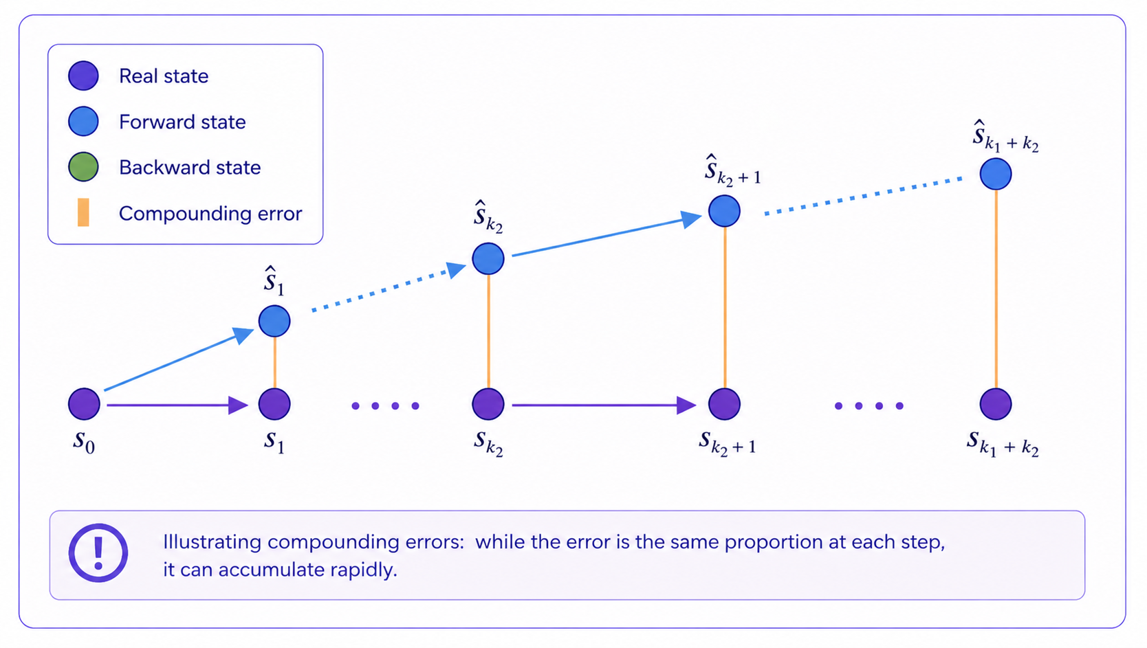
Compounding error

Prediction errors accumulate rapidly as planning horizon length increases. Even small per-step inaccuracies, whether from systematic bias, distribution shift, or model imprecision, can, if not corrected, cause the planned trajectory to drift into parts of the state space where the model hasn't been trained and is therefore least reliable.

Practical mitigations include shorter planning horizons, model ensembles that flag unreliable predictions via disagreement, and uncertainty-aware planning strategies that steer clear of unreliable regions.

Model uncertainty

Model-based RL faces two kinds of uncertainty.

Epistemic uncertainty reflects situations where the learned model was not exposed to state-action pairs for a specific region of the environment during training; it can often be reduced by collecting more targeted rollouts.

Aleatoric uncertainty reflects irreducible randomness in the environment, such as noisy observations or stochastic transitions, and persists even with abundant data.

In practice, a simple baseline is the use of ensembles: train multiple dynamics models to leverage their disagreement as an uncertainty signal during planning. This allows for high-disagreement areas to be avoided in favor of shortened horizons, or as a sign to trigger frequent replanning.

If the environment is highly stochastic, a robust practical solution is to use probabilistic dynamic models, where the training objective allows predictions to be made as a probability distribution.

Distribution shift

Even with a strong dynamics model, it can be challenging to maintain performance when applied to states outside the training distribution. As the policy improves, it often reaches novel regions the model hasn't seen, leading to unreliable predictions and compounding planning errors.

An effective mitigation is iterative retraining: 

1. Collect rollouts from the current policy
2. Retrain the model to capture new regions
3. Repeat. 

For robust use, iterative optimization can be triggered using metrics obtained by monitoring model error.

Model-based RL patterns in LLM development

Model-based RL patterns appear in LLM development under different names, and some are analogies rather than strict implementations. The shared idea is using a learned model to actively guide decisions by evaluating candidates, selecting among them, or generating synthetic experience. This differs from model-free methods, where a reward model provides the training signal but does not guide search or selection directly.

‍

Reward models as learned evaluators

Reward models can be deployed as preference predictors that score outputs. Unlike dynamics models, they don't predict transitions, but they evaluate whether the outcome was optimal.

Reward models also appear in model-free methods like PPO, where they provide the training signal for policy updates. The model-based connection is specifically when they are used to drive search or selection over candidates.

‍

What they enable is the ability to search without a human in the loop. You can:

1. Generate candidate responses
2. Score them automatically
3. Select the option that yields the highest predicted reward. 

The reward model acts as a learned utility function to enable automated evaluation.

Dynamics models are trained to accurately predict what will happen given the action taken, regardless of whether that action is optimal. Reward models are trained to assess the quality of the action, based on whether the state it leads to is optimal.

Best-of-N as search/reranking

The Best-of-N approach generates N candidate responses, scores each with a reward model, and selects the highest-scoring option.

This is a one-step search or reranking rather than multi-step planning; the model-based RL analogy is that of using a learned evaluator to select among sampled options.

A common risk is reward hacking, where the model exploits imperfections in the reward signal, underscoring the need for calibration checks and verifiable signals. Compute cost also scales with N, adding another constraint. 

Process reward models (PRMs) as dense evaluators

PRMs provide step-by-step scores over reasoning traces, enabling credit assignment. They allow identification of which reasoning step failed rather than just knowing the final answer was wrong.

The model-based RL analogy is that dense reward signals enable more effective search over reasoning trajectories. It's worth noting that PRMs evaluate steps; they don't predict transitions, so they remain evaluators rather than predictive dynamic models.

Synthetic data as model-generated experience

The underlying pattern uses a learned model to generate synthetic experience. Candidate outputs are produced, verified for correctness, and the successes are retained as training data. An example is DeepSeek R1, which applies rejection sampling from an RL-trained checkpoint to collect high-quality examples for supervised fine-tuning. In rejection sampling, multiple candidate outputs are generated and filtered through a correction check, retaining only the successful ones. 

The model-based RL analogy is that of imagined rollouts augmenting real collected data, where the model (in this case, the LLM itself) generates additional training signals.

Applying model-based RL concepts to text generation

The following example applies the core model-based RL insight to text generation: use a learned model to evaluate options before committing. The implementation uses a value predictor rather than a dynamics model.

1. A value predictor trained on scored examples estimates response quality from partial outputs
2. Look-ahead search generates partial candidates, scores them with the value predictor, and continues the most promising ones
3. An iterative self-training loop retrains both the predictor and the policy on new data. 

The pipeline generates candidate responses, scores them with a reward model, trains a value predictor on that data, and compares value-guided generation against standard Best-of-N sampling under matched compute budgets.

Note: The code for this article is available in this Google Colab Notebook.

Install and import libraries

!pip install transformers trl datasets accelerate sentence-transformers scikit-learn peft

import torch
import numpy as np
from transformers import AutoModelForCausalLM, AutoTokenizer, pipeline
from trl import SFTTrainer, SFTConfig
from peft import LoraConfig
from datasets import Dataset
from sentence_transformers import SentenceTransformer
from sklearn.linear_model import Ridge

Load base and reward models

Two models form the foundation: one generates, the other evaluates. 

1. The policy model (Qwen2.5-1.5B-Instruct) generates candidate responses. 
2. A separate reward model (DeBERTa-based, trained on human preferences) provides automated quality scores, replacing the need for human evaluation on every output. 

The reward model is a learned evaluator optimized to predict quality, rather than a dynamics model that predicts state transitions.

model = AutoModelForCausalLM.from_pretrained(
    "Qwen/Qwen2.5-1.5B-Instruct",
    dtype=torch.float16,
    device_map="auto",
)
tokenizer = AutoTokenizer.from_pretrained("Qwen/Qwen2.5-1.5B-Instruct")
if tokenizer.pad_token is None:
    tokenizer.pad_token = tokenizer.eos_token

reward_pipeline = pipeline(
    "text-classification",
    model="OpenAssistant/reward-model-deberta-v3-large-v2",
    device_map="auto",
)

‍

Define generation and scoring functions

Two functions provide the foundation for everything that follows. 

1. generate_candidates produces multiple response options for a given prompt using temperature-based sampling. It introduces diversity so the system has meaningfully different trajectories to evaluate. 
2. score_responses passes each candidate through the reward model to obtain a quality score.

def generate_candidates(prompt, n=4, max_new_tokens=256, temperature=0.7):
    """Generate n candidate responses for a prompt."""
    messages = [{"role": "user", "content": prompt}]
    formatted = tokenizer.apply_chat_template(
        messages, tokenize=False, add_generation_prompt=True
    )
    inputs = tokenizer(formatted, return_tensors="pt").to(model.device)

    with torch.no_grad():
        outputs = model.generate(
            **inputs,
            max_new_tokens=max_new_tokens,
            num_return_sequences=n,
            do_sample=True,
            temperature=temperature,
            pad_token_id=tokenizer.eos_token_id,
        )

    input_length = inputs["input_ids"].shape[1]
    return [
        tokenizer.decode(out[input_length:], skip_special_tokens=True).strip()
        for out in outputs
    ]


def score_responses(prompt, responses):
    """Score responses using the reward model."""
    scores = []
    for response in responses:
        text = f"User: {prompt}\nAssistant: {response}"
        result = reward_pipeline(text, truncation=True, max_length=512)
        scores.append(result[0]["score"])
    return scores

Collect scored data

For each prompt, multiple candidate responses are generated and scored with the reward model. The full set of scored examples, including low-quality responses and not just the best, provides the training data for the quality predictor. Learning from the full score spectrum allows the predictor to distinguish between promising and unpromising trajectories.

This data collection step is the generation phase of rejection sampling: 

1. Generate multiple candidate outputs
2. Score them
3. Keep only those that meet a quality threshold. 

Here, all scored examples are retained. The threshold-based filtering is applied later during data selection for policy fine-tuning.

prompts = [
    "Explain what a neural network is.",
    "What are the benefits of exercise?",
    "How does photosynthesis work?",
    "What is machine learning?",
    "Why is the sky blue?",
]

scored_data = []
for prompt in prompts:
    candidates = generate_candidates(prompt, n=4)
    scores = score_responses(prompt, candidates)
    for response, score in zip(candidates, scores):
        scored_data.append({
            "prompt": prompt,
            "response": response,
            "score": score,
        })

Learn a quality predictor (value estimator)

The quality predictor is a value estimator. Given a prompt and the beginning of a response, it predicts the expected reward of the eventual full output. It does not predict state transitions. The distinguishing factor is that decisions are made during generation, not only after completion.

This is what enables look-ahead planning: rather than generating complete responses before evaluating them, the predictor assesses partial trajectories mid-generation, allowing the system to focus compute resources on the most promising directions.

The predictor trains on prefixes of previously scored responses. A sentence embedding model (all-MiniLM-L6-v2) maps each prompt-plus-prefix pair to a dense vector. Ridge regression learns the mapping from the embeddings to reward model scores.

class QualityPredictor:
    def __init__(self, embedding_model_name="all-MiniLM-L6-v2"):
        self.embedder = SentenceTransformer(embedding_model_name)
        self.regressor = Ridge(alpha=1.0)
        self.is_trained = False

    def _embed(self, prompt, response_text):
        combined = f"Prompt: {prompt}\nResponse: {response_text}"
        return self.embedder.encode(combined)

    def train(self, scored_data, prefix_ratio=0.5):
        if len(scored_data) < 2:
            print(f"Warning: Only {len(scored_data)} examples -- need >= 2. Skipping.")
            return

        embeddings, scores = [], []
        for item in scored_data:
            words = item["response"].split()
            prefix_len = max(1, int(len(words) * prefix_ratio))
            prefix = " ".join(words[:prefix_len])
            embeddings.append(self._embed(item["prompt"], prefix))
            scores.append(item["score"])

        X = np.array(embeddings)
        if X.ndim == 1:
            X = X.reshape(1, -1)
        self.regressor.fit(X, np.array(scores))
        self.is_trained = True

    def predict(self, prompt, partial_response):
        emb = self._embed(prompt, partial_response).reshape(1, -1)
        return float(self.regressor.predict(emb)[0])

Planned generation with look-ahead search

Look-ahead search evaluates partial candidates to estimate their future quality prior to full completion, using the trained quality predictor. Rather than generating complete responses and filtering after the fact, partial candidates are produced and scored, enabling the search process to prioritize and expand the most promising trajectories.

The value predictor scores partial outputs mid-generation, allowing the system to focus resources on the most promising directions.

1. Simulate partial trajectories forward
2. Evaluate them using the learned value predictor
3. Commit to the best branches
4. Continue generation from there. 

The prefix length of 64 tokens is a practical default for this example, short enough to limit prediction drift (the shorter the prefix, the less the value estimate can diverge from actual quality) while still long enough for the predictor to make meaningful quality estimates.  It is a tunable parameter. Shorter prefixes suit open-ended generation where early divergence matters, longer prefixes suit structured outputs where more context improves prediction accuracy.

def generate_partial(prompt, n=4, max_tokens=64):
    """Generate partial responses (first max_tokens tokens only)."""
    messages = [{"role": "user", "content": prompt}]
    formatted = tokenizer.apply_chat_template(
        messages, tokenize=False, add_generation_prompt=True
    )
    inputs = tokenizer(formatted, return_tensors="pt").to(model.device)

    with torch.no_grad():
        outputs = model.generate(
            **inputs,
            max_new_tokens=max_tokens,
            num_return_sequences=n,
            do_sample=True,
            temperature=0.9,
            pad_token_id=tokenizer.eos_token_id,
        )

    input_length = inputs["input_ids"].shape[1]
    return [
        tokenizer.decode(out[input_length:], skip_special_tokens=True).strip()
        for out in outputs
    ]


def continue_from_partial(prompt, partial_text, n=2, max_tokens=192):
    """Continue generation from a partial response."""
    messages = [{"role": "user", "content": prompt}]
    continued_prompt = tokenizer.apply_chat_template(
        messages, tokenize=False, add_generation_prompt=True
    )
    continued_prompt += partial_text
    inputs = tokenizer(continued_prompt, return_tensors="pt").to(model.device)

    with torch.no_grad():
        outputs = model.generate(
            **inputs,
            max_new_tokens=max_tokens,
            num_return_sequences=n,
            do_sample=True,
            temperature=0.7,
            pad_token_id=tokenizer.eos_token_id,
        )

    input_length = inputs["input_ids"].shape[1]
    return [
        (partial_text + tokenizer.decode(out[input_length:],
         skip_special_tokens=True)).strip()
        for out in outputs
    ]


def planned_generation(prompt, predictor, n_branches=4,
                       prefix_tokens=64, continuations_per_branch=2):
    """Value-guided generation with look-ahead search"""
    # Fallback if predictor not yet trained
    if not predictor.is_trained:
        candidates = generate_candidates(prompt, n=n_branches)
        scores = score_responses(prompt, candidates)
        best_idx = scores.index(max(scores))
        return candidates[best_idx], scores[best_idx], []

    # Step 1: Generate partial candidates (simulate forward)
    partials = generate_partial(prompt, n=n_branches, max_tokens=prefix_tokens)

    # Step 2: Score partials with learned predictor (evaluate)
    predicted_scores = [predictor.predict(prompt, p) for p in partials]

    # Step 3: Select top branches (commit to best trajectories)
    ranked = sorted(zip(partials, predicted_scores),
                    key=lambda x: x[1], reverse=True)
    top_partials = [p for p, s in ranked[:2]]

    # Step 4: Continue generation from selected branches
    full_responses = []
    for partial in top_partials:
        continuations = continue_from_partial(
            prompt, partial, n=continuations_per_branch
        )
        full_responses.extend(continuations)

    # Step 5: Final scoring with real reward model
    scores = score_responses(prompt, full_responses)
    best_idx = scores.index(max(scores))
    return full_responses[best_idx], scores[best_idx], predicted_scores

Comparison: Best-of-N vs. planned generation

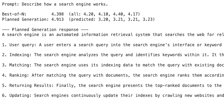
To evaluate whether the quality predictor adds value, the implementation compares Planned Generation against Best-of-N under a matched compute budget. 

Best-of-N generates four complete responses (256 tokens each) and picks the highest-scoring one. Planned generation splits the same budget differently: four partial responses (64 tokens each), scored by the quality predictor to select the two most promising branches, then two completions per branch (192 tokens each), scored by the reward model to select the best. 

Both approaches produce roughly 1,024 total tokens and make four reward model calls; the only difference is whether the quality predictor guides branch selection during generation.

def best_of_n(prompt, n=4):
    """Generate n complete responses and pick the highest-scoring one."""
    candidates = generate_candidates(prompt, n=n)
    scores = score_responses(prompt, candidates)
    best_idx = scores.index(max(scores))
    return candidates[best_idx], scores[best_idx], scores

Running both methods on the same five prompts reveals per-prompt scores, win counts, and a side-by-side response comparison. Testing on an unseen prompt further evaluates whether the quality predictor generalizes beyond the topics it was trained on. 

If the predictor has learned a useful relationship between partial response content and final reward, its informed pruning produces higher-scoring completions than blind generation.

Here is the output: 

Iterative training loop

So far, the value predictor guides branch selection, with the policy itself remaining fixed. The full pipeline closes this loop by iterating between three steps:

1. Planned data collection: Use the quality predictor to guide generation, producing new scored examples that expand the dataset.
2. Predictor retraining (model learning): Retrain the quality predictor on the expanded dataset to improve its ability to evaluate partial trajectories.
3. Policy update: Fine-tune the LLM via LoRA on high-quality, filtered data to improve the quality of base generations for the next iteration.

This follows the expert iteration pattern: generate with the current policy, score and filter, retrain on the best outputs. Each iteration addresses distribution shift: as the policy improves, the predictor is retrained on data from the updated policy, keeping the value estimates aligned with the current generation distribution.

Steps 1 and 2 work at any data scale. Step 3, however, requires enough prompt diversity for the model to generalize rather than memorize. 

With only five prompts, the model overfits to a narrow topic distribution, which is expected behavior at this scale. For context, real iterative training systems operate with far larger datasets:

• STaR (Zelikman et al., 2022): 7,500+ problems across 16-36 iterations
• ReST-EM (Singh et al., 2023): 7,500 problems with 32 solutions generated per problem per iteration
• DeepSeek R1 (2025): approximately 800,000 examples for the supervised fine-tuning stage

For this reason, the policy update code is provided as a ready-to-use template that can be run directly once a suitable prompt dataset is available (500+ diverse prompts recommended). The LoRA configuration updates only the attention projection weights.

trainer = SFTTrainer(
    model=model,
    args=SFTConfig(
        output_dir="./trained_model",
        num_train_epochs=1,
        per_device_train_batch_size=1,
        gradient_accumulation_steps=4,
        learning_rate=2e-4,
        logging_steps=10,
        save_strategy="no",
        report_to="none",
        max_length=512,
    ),
    train_dataset=train_dataset,
    peft_config=LoraConfig(
        r=16, lora_alpha=32,
        target_modules=["q_proj", "v_proj"],
        task_type="CAUSAL_LM",
    ),
    processing_class=tokenizer,
)
trainer.train()

‍

To use the loop with your own data, replace the example prompts with a task-specific prompt dataset (500+ diverse prompts recommended) and run Steps 1–3 for each self-training iteration.

Recommendations

Consider the following.

Best-of-N for scaling evaluation

When human judges can't feasibly evaluate every output, a learned reward model allows evaluation to scale.

Generate multiple candidates and select the highest-scoring one at inference time. It provides a practical path to optimizing output quality without requiring proportional increases in human evaluation effort.

GRPO and verifiable rewards

If correctness is easily verifiable, such as code that passes tests or math answers that match ground truth, model-free approaches like GRPO with verifiable rewards are typically simpler and avoid the challenges inherent in learning accurate reward predictors.

When the reward signal is reliable and cheap to compute, the added complexity of learned evaluators may not be warranted.

Process reward models for reasoning chains

When sequence and credit assignment matter, particularly when you need to identify which step in a reasoning chain failed, PRMs provide the dense feedback signal needed to guide search over trajectories.

This becomes especially relevant for mathematical reasoning and other domains where intermediate steps matter as much as final answers.

Hybrid approaches in production

A common pattern in production is to train with model-free RL, which is typically cheaper and simpler, then deploy with model-based inference-time search. It yields better output quality when compute budget allows.

Many production systems prefer hybrid approaches, using each where it provides the most benefit.

Decision framework

‍

How Patronus AI helps

The model-based RL patterns discussed in this article, particularly reward models and Best-of-N sampling, depend on one critical factor: the quality of evaluation signals.

When those signals are unreliable or are exploited by an agent, it is difficult to obtain successful results. Patronus AI provides RL environments with auditable, automated reward signals for LLM evaluation and training.

Patronus environments use objective correctness checks. These deterministic signals are reproducible and auditable, reducing the variance and inconsistency common to subjective evaluations.

Patronus supported environment types

Patronus ships with pre-built RL environments spanning common production domains that include tools for:

• Coding tasks to generate and correct program outputs
• SQL and database Q&A agents that query structured data
• Customer service agents
• Finance Q&A agents that surface insights from financial data
• Trading agents that interact with markets or simulated UIs
• Web interface navigation agents for review or e-commerce workflows.

Each environment includes structured tasks and built-in evaluation logic that checks not only correctness but also procedural order, error conditions, tool usage, and consistency. Visit Patronus AI to learn more about the range of helpful tools available to assist with building your own customized RL environment.

{{banner-dark-small-1-rle="/banners"}}

Conclusion

Model-based reinforcement learning is an elegant approach to training agents that uses a learned dynamics model to imagine the outcomes of possible actions. It is an excellent choice for AI systems executing complex tasks. However, there are various challenges when building advanced autonomous systems.  

Platforms like Patronus AI offer tools to address these challenges effectively when building intelligent systems with model-based RL, enabling solutions tailored to specific environments. 

The dynamics model at the heart of this article is also the starting point of a larger research direction, i.e., world models. World models extend transition and reward prediction into complete learned simulators of an environment, accurate enough that agents like DreamerV3 can be trained largely on imagined experience. The concepts covered here, from planning with a learned model to managing compounding error, are the foundations on which world models build at scale.